Rate Limiter Algorithms
Algorithms for rate limiting
The task of a rate limiter is directed by highly efficient algorithms, each of which has distinct advantages and disadvantages. However, there is always a choice to choose an algorithm or combination of algorithms depending on what we need at a given time. While different algorithms are used in addition to those below, we’ll take a look at the following popular algorithms.
- Token bucket
- Leaking bucket
- Fixed window counter
- Sliding window log
- Sliding window counter
Token bucket algorithm
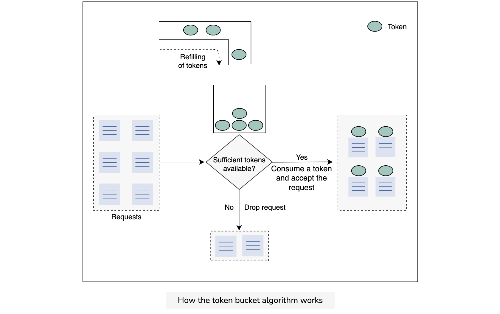
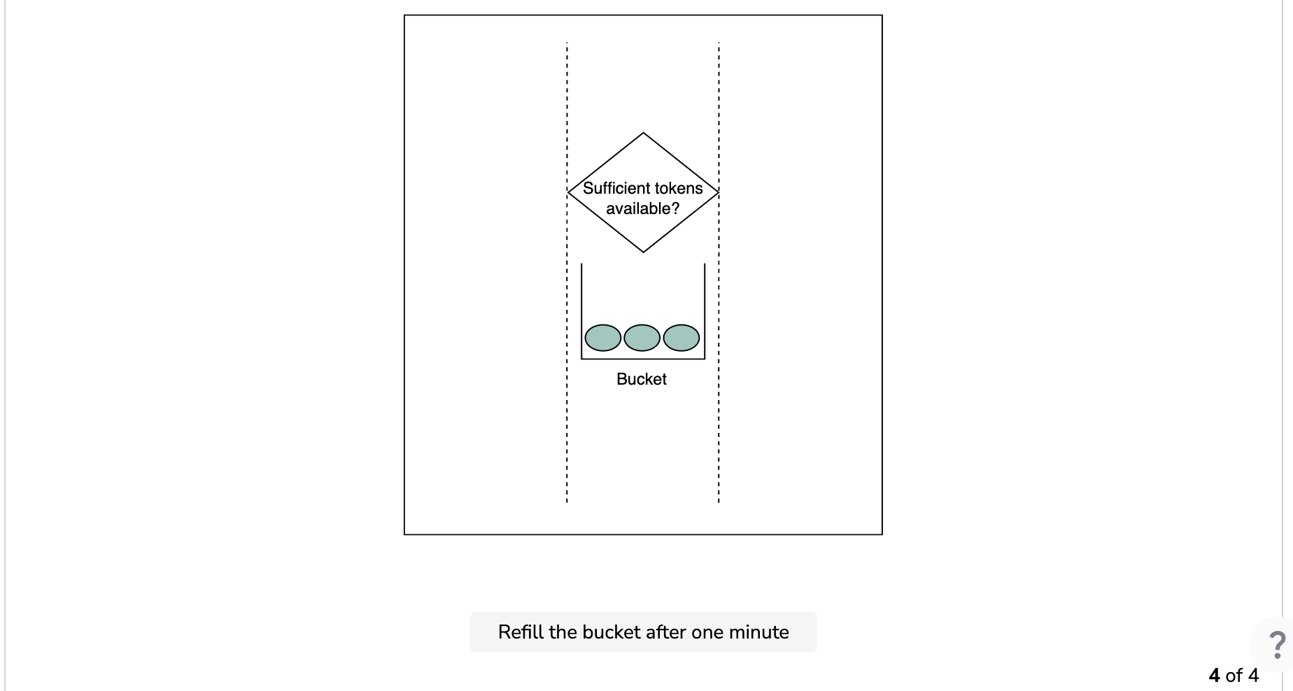
This algorithm uses the analogy of a bucket with a predefined capacity of tokens. The bucket is periodically filled with tokens at a constant rate. A token can be considered as a packet of some specific size. Hence, the algorithm checks for the token in the bucket each time we receive a request. There should be at least one token to process the request further.
The flow of the token bucket algorithm is as follows:
Assume that we have a predefined rate limit of R and the total capacity of the bucket is C.
- The algorithm adds a new token to the bucket after every 1R1 seconds.
- The algorithm discards the new incoming tokens when the number of tokens in the bucket is equal to the total capacity C of the bucket.
- If there are N incoming requests and the bucket has at least N tokens, the tokens are consumed, and requests are forwarded for further processing.
- If there are N incoming requests and the bucket has a lower number of tokens, then the number of requests accepted equals the number of available tokens in the bucket.
The following illustration represents the working of the token bucket algorithm.
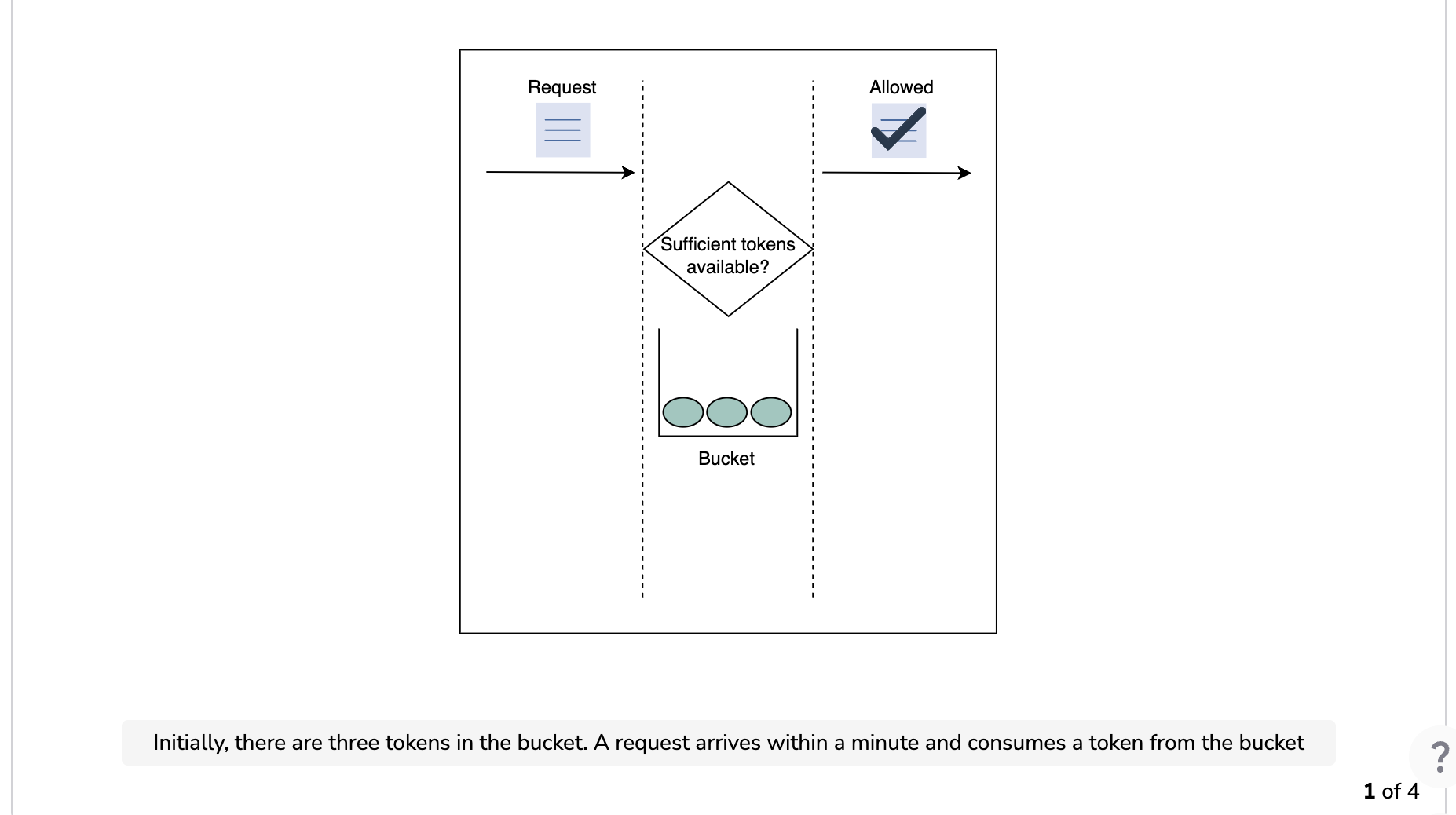
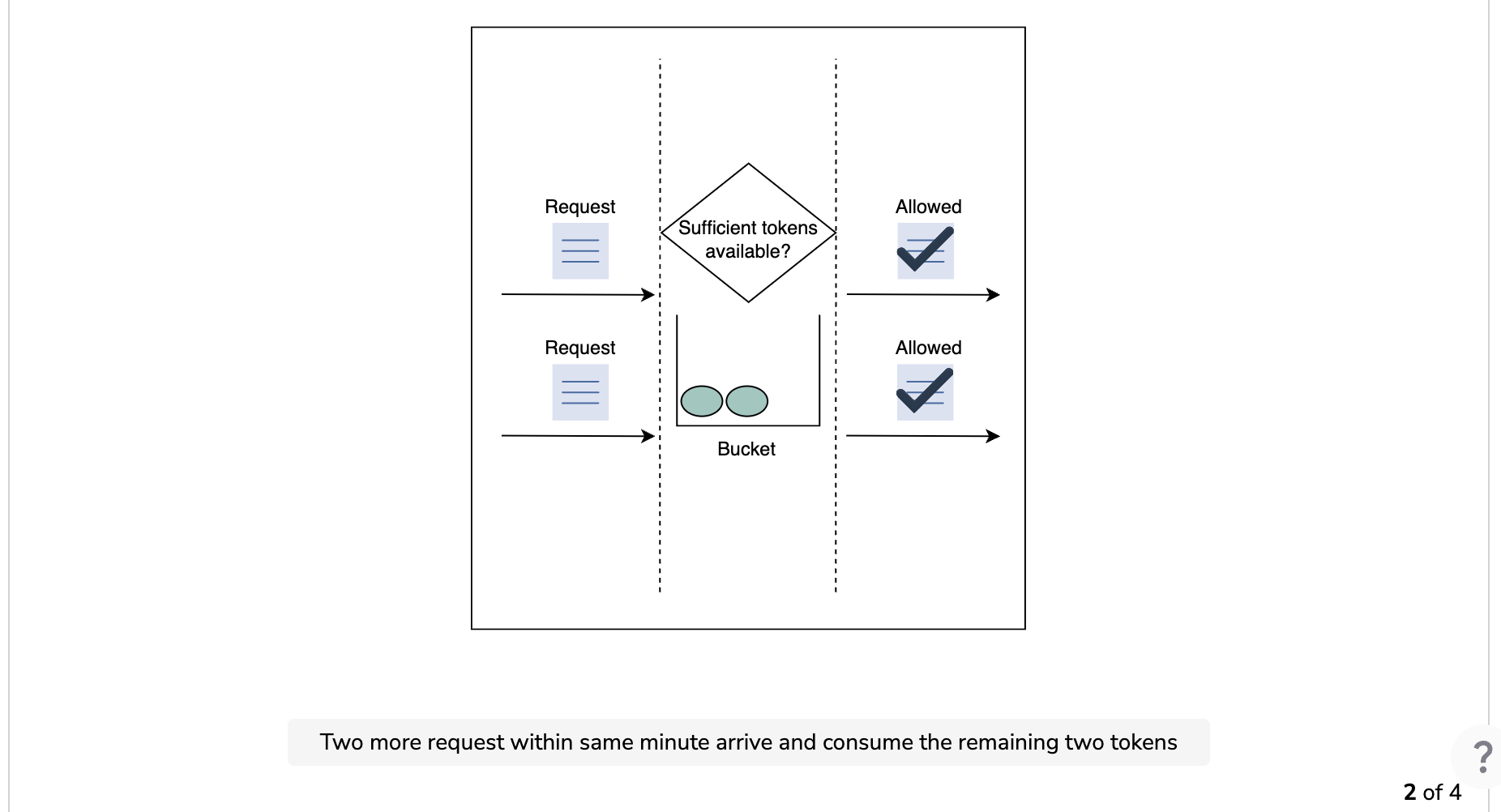
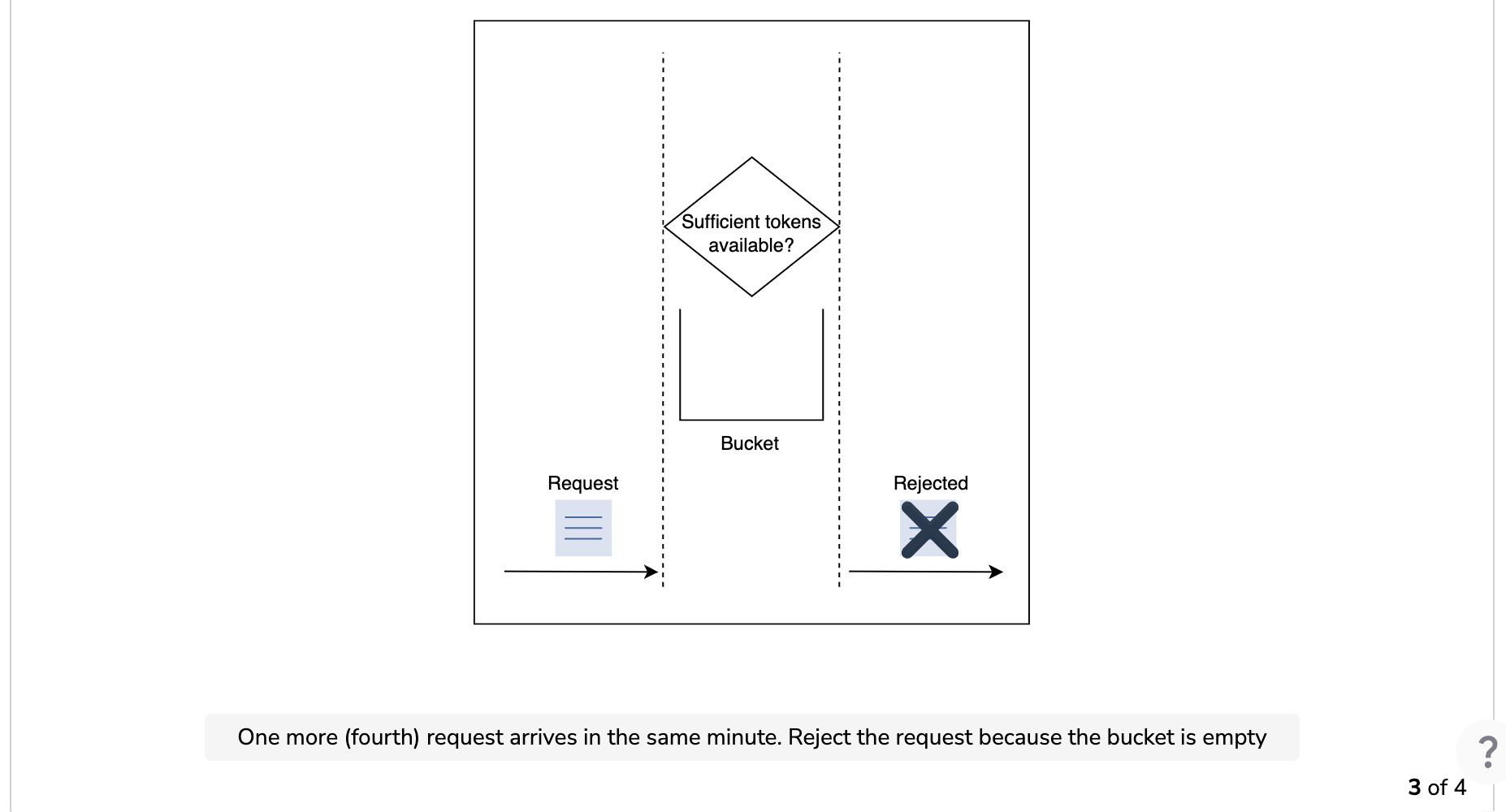
The following illustration demonstrates how token consumption and rate-limiting logic work. In this example, the capacity of the bucket is three, and it is refilled at a rate of three tokens per minute.
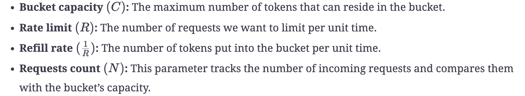
Essential parameters
We require the following essential parameters to implement the token bucket algorithm:
Advantages
- This algorithm can cause a burst of traffic as long as there are enough tokens in the bucket.
- It is space efficient. The memory needed for the algorithm is nominal due to limited states.
Disadvantages
- Choosing an optimal value for the essential parameters is a difficult task.
Point to Ponder
Question
Apart from permitting bursts, can the token bucket algorithm surpass the limit at the edges?
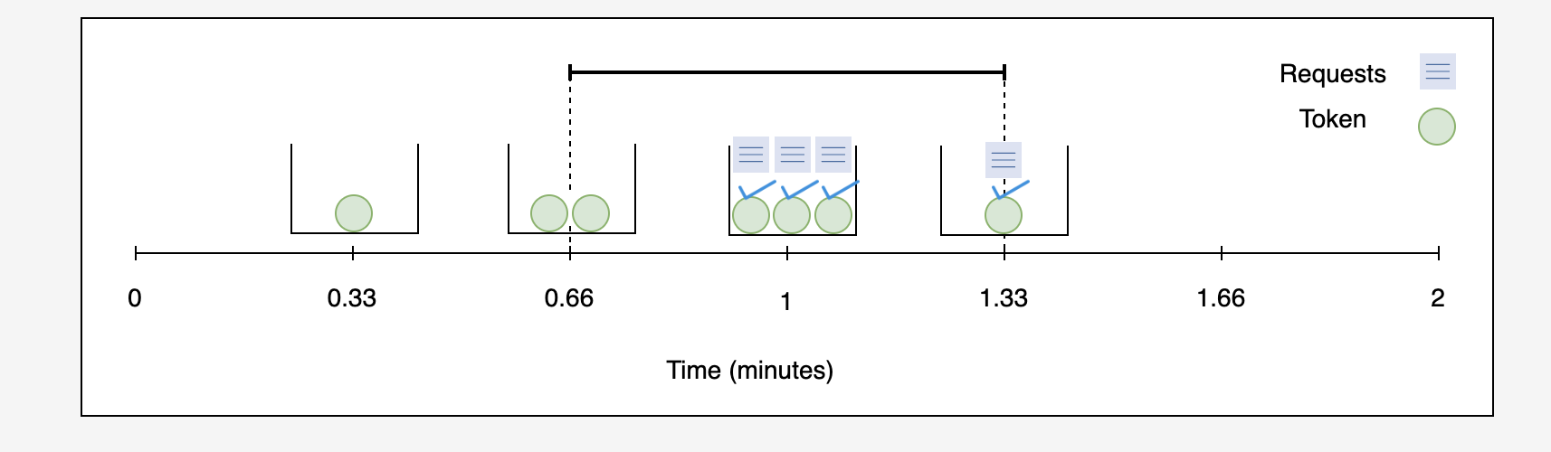
Yes, the token bucket algorithm can sometimes suffer from overrunning the limit at the edges, as demonstrated by the following example:
Consider a scenario with a bucket capacity equal to 33, and the number of requests allowed per minute is also 33. This yields a refill rate of 0.330.33 minutes, which means that a new token will come every 0.330.33 minute.
In the illustration below, three tokens have been accumulated at the end of the first minute. At the same time, a burst of requests arrives and consumes all three tokens, leaving the bucket empty. At the end of 1.331.33 minutes (at a refill rate of 0.330.33), a new token is added to the bucket. Simultaneously, a new request arrives and consumes the token.
However, if we consider the duration from 0.660.66 to 1.331.33 minutes, we’ll see that a total of four tokens have been consumed.
This example shows that the token bucket can surpass the limit at the edges.
-----------
The leaking bucket algorithm
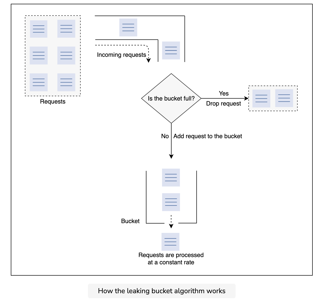
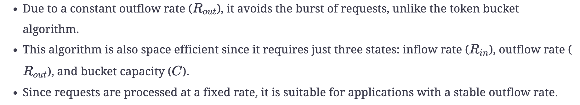
The leaking bucket algorithm is a variant of the token bucket algorithm with slight modifications. Instead of using tokens, the leaking bucket algorithm uses a bucket to contain incoming requests and processes them at a constant outgoing rate. This algorithm uses the analogy of a water bucket leaking at a constant rate. Similarly, in this algorithm, the requests arrive at a variable rate. The algorithm process these requests at a constant rate in a first-in-first-out (FIFO) order.
Let’s look at how the leaking bucket algorithm works in the illustration below:
Essential parameters
The leaking bucket algorithm requires the following parameters.
.png)
Advantages
Disadvantages
- A burst of requests can fill the bucket, and if not processed in the specified time, recent requests can take a hit.
- Determining an optimal bucket size and outflow rate is a challenge.
Fixed window counter algorithm
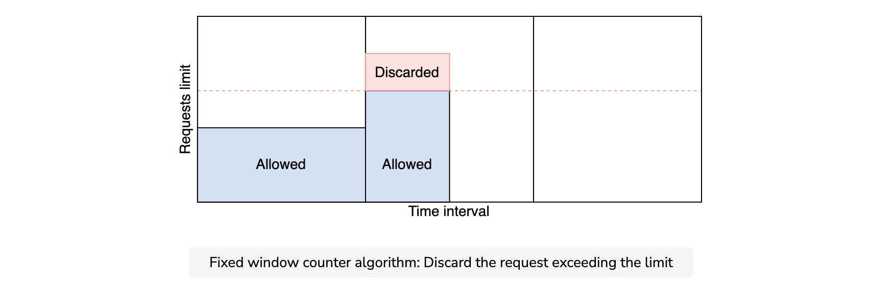
This algorithm divides the time into fixed intervals called windows and assigns a counter to each window. When a specific window receives a request, the counter is incremented by one. Once the counter reaches its limit, new requests are discarded in that window.
As shown in the below figure, a dotted line represents the limit in each window. If the counter is lower than the limit, forward the request; otherwise, discard the request.
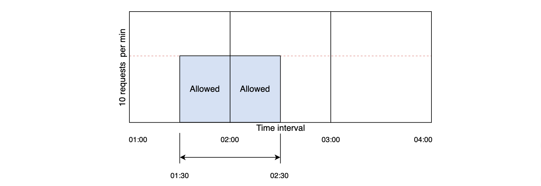
There is a significant problem with this algorithm. A burst of traffic greater than the allowed requests can occur at the edges of the window. In the below figure, the system allows a maximum of ten requests per minute. However, the number of requests in the one-minute window from 01:30 to 02:30 is 20, which is greater than the allowed number of requests.
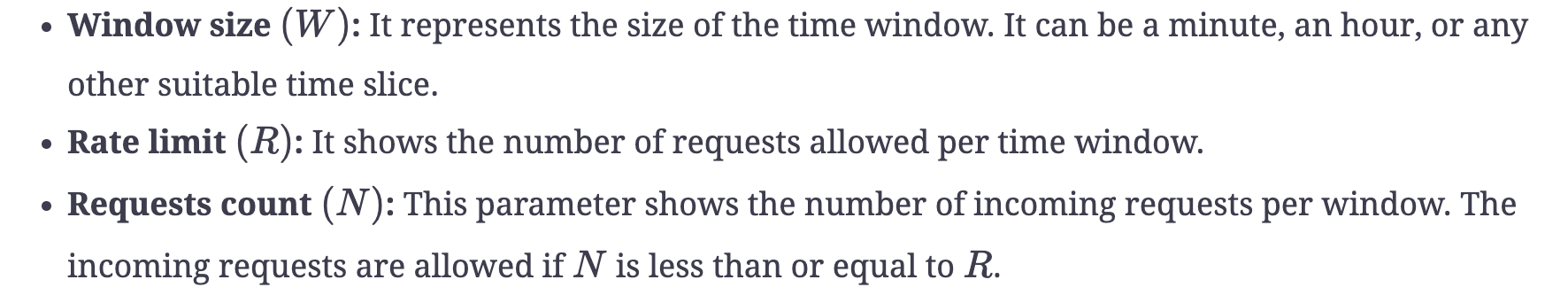
Essential parameters
The fixed window counter algorithm requires the following parameters:
Advantages
- It is also space efficient due to constraints on the rate of requests.
- As compared to token bucket-style algorithms (that discard the new requests if there aren’t enough tokens), this algorithm services the new requests.
Disadvantages
- A consistent burst of traffic (twice the number of allowed requests per window) at the window edges could cause a potential decrease in performance.
Sliding window log algorithm
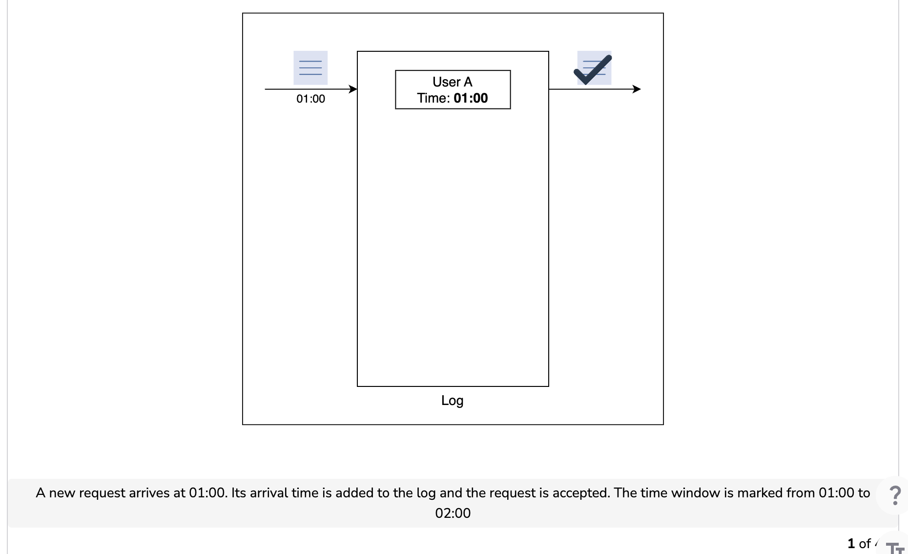
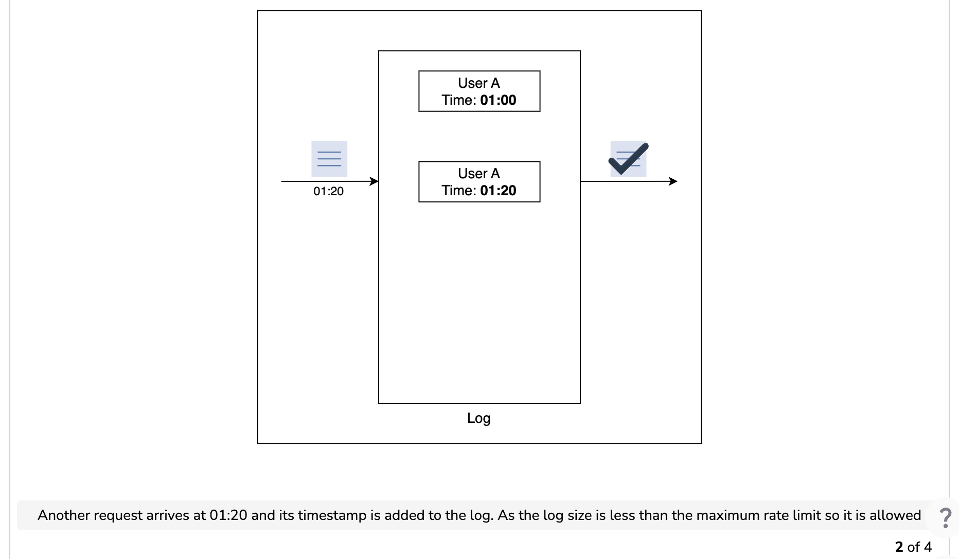
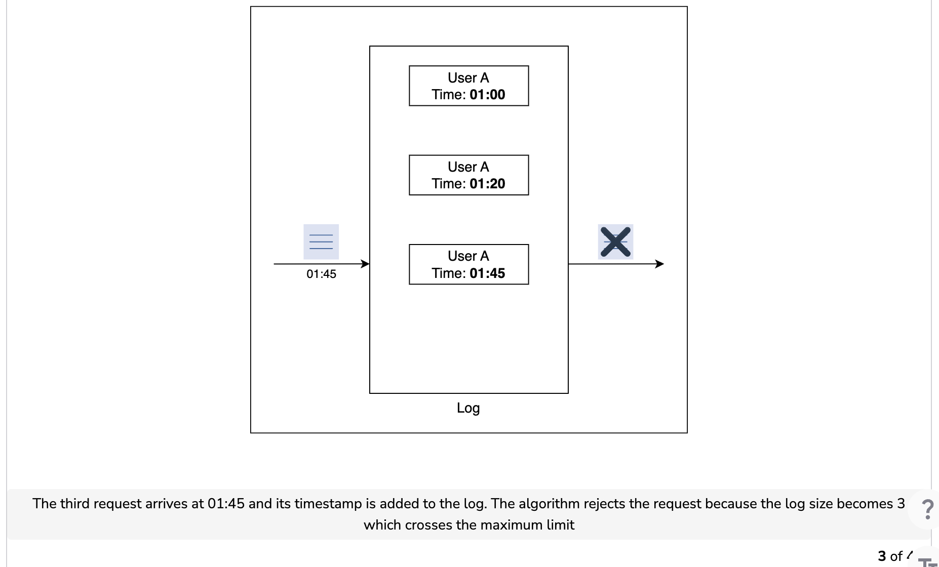
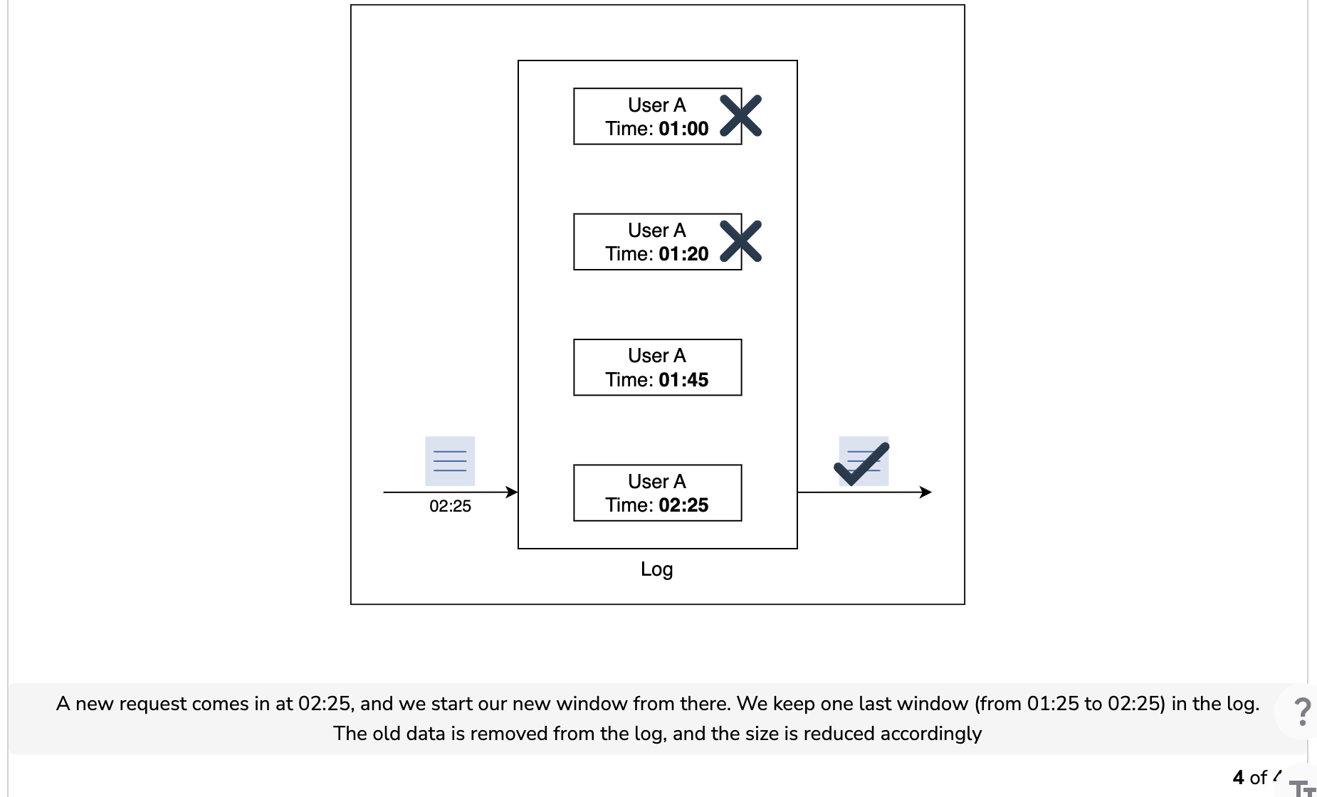
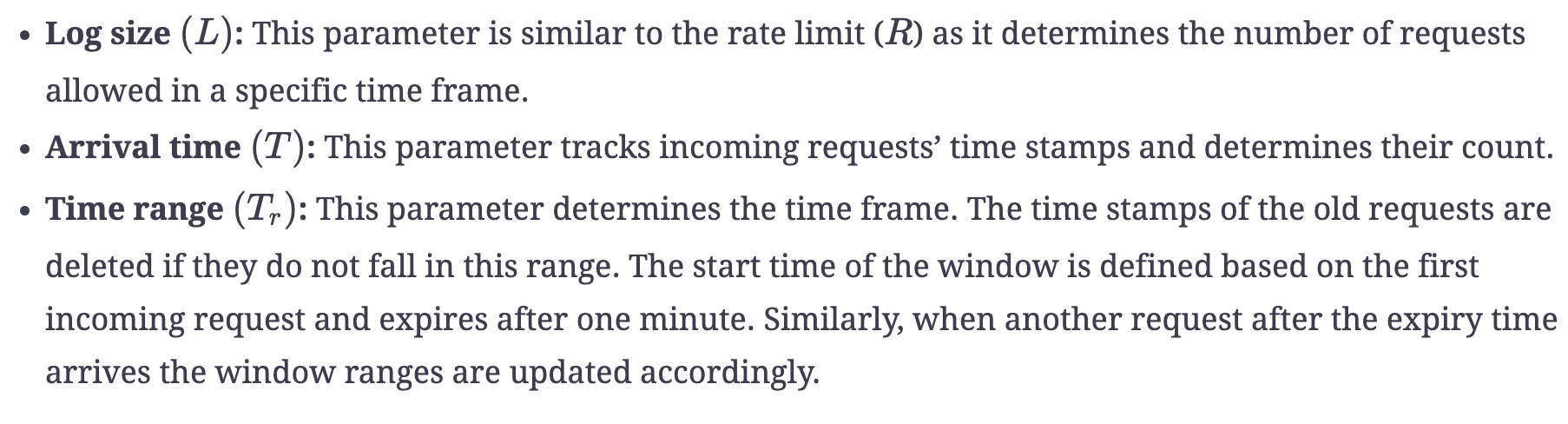
The sliding window log algorithm keeps track of each incoming request. When a request arrives, its arrival time is stored in a hash map, usually known as the log. The logs are sorted based on the time stamps of incoming requests. The requests are allowed depending on the size of the log and arrival time.
The main advantage of this algorithm is that it doesn’t suffer from the edge conditions, as compared to the fixed window counter algorithm.
Let’s understand how the sliding window log algorithm works in the illustration below. Assume that we have a maximum rate limit of two requests in a minute.
Essential parameters
The following parameters are required to implement the sliding window log algorithm:
Advantages
- The algorithm doesn’t suffer from the boundary conditions of fixed windows.
Disadvantages
- It consumes extra memory for storing additional information, the time stamps of incoming requests. It keeps the time stamps to provide a dynamic window, even if the request is rejected.
Sliding window counter algorithm
Unlike the previously fixed window algorithm, the sliding window counter algorithm doesn’t limit the requests based on fixed time units. This algorithm takes into account both the fixed window counter and sliding window log algorithms to make the flow of requests more smooth. Let’s look at the flow of the algorithm in the below figure.
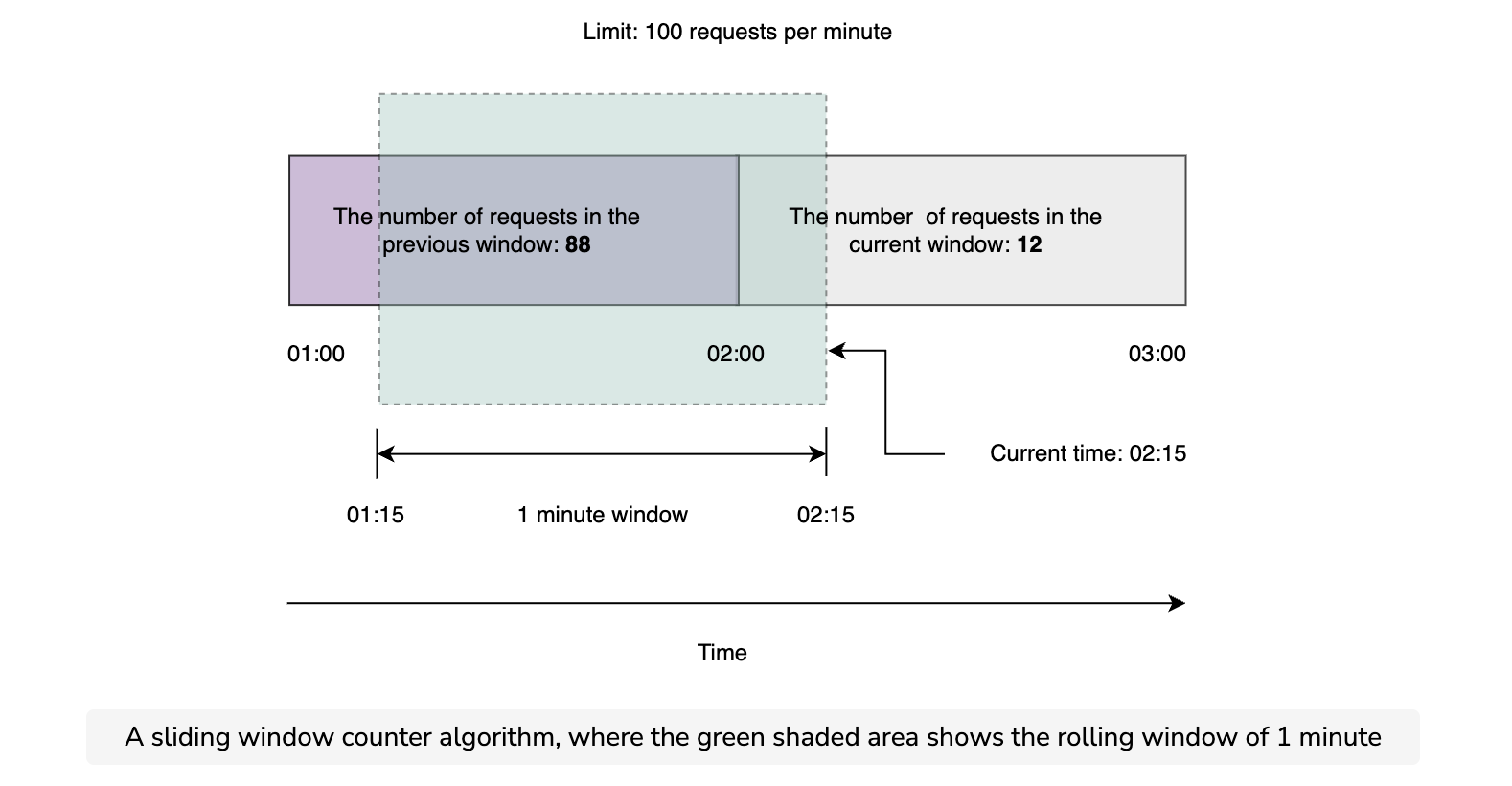
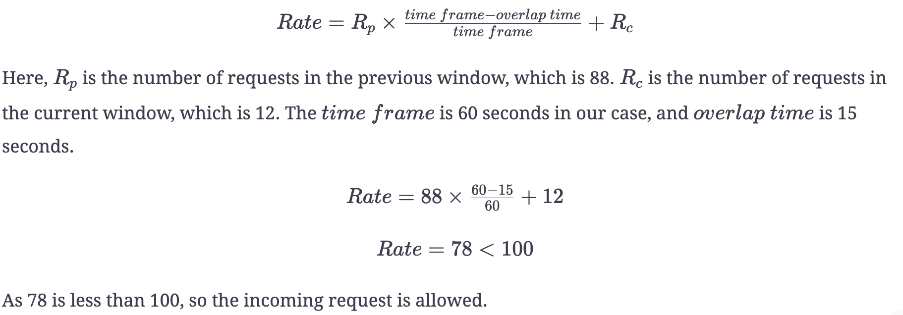
In the above figure, we’ve 88 requests in the previous window while 12 in the current window. We’ve set the rate limit to 100 requests per minute. Further, the rolling window overlaps 15 seconds with the current window. Now assume that a new request arrives at 02:15. We’ll decide which request to accept or reject using the mathematical formulation:
Essential parameters
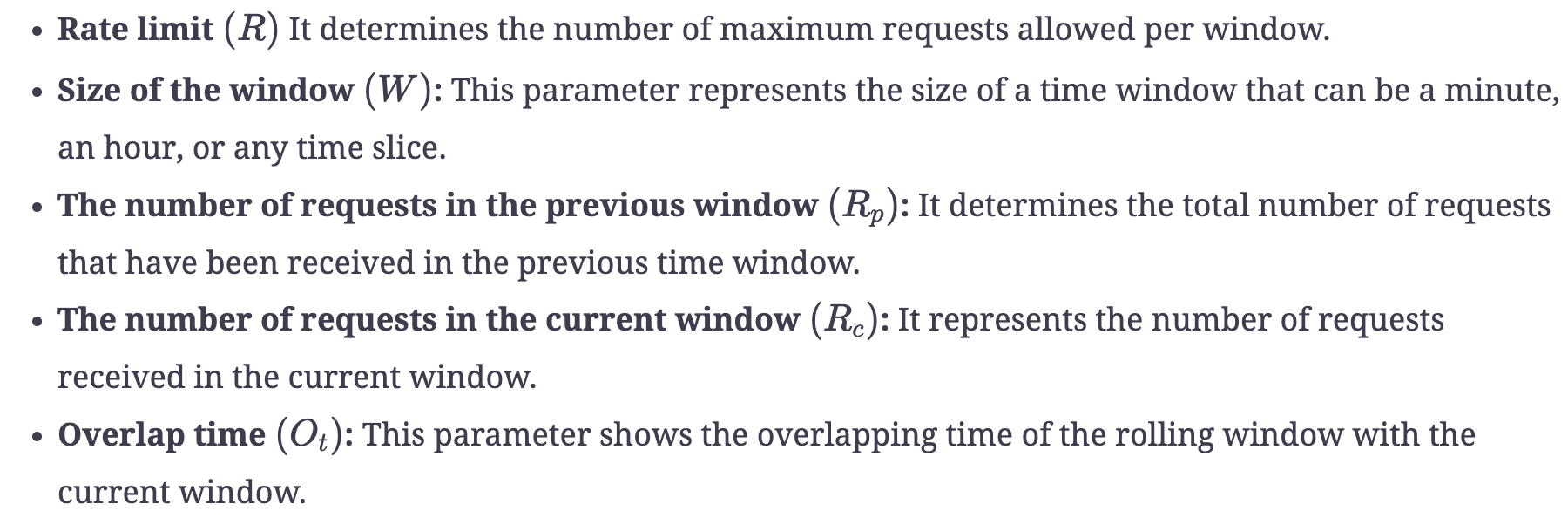
This algorithm is relatively more complex than the other algorithms described above. It requires the following parameters:
Advantages
- The algorithm is also space efficient due to limited states: the number of requests in the current window, the number of requests in the previous window, the overlapping percentage, and so on.
- It smooths out the bursts of requests and processes them with an approximate average rate based on the previous window.
Disadvantages
- This algorithm assumes that the number of requests in the previous window is evenly distributed, which may not always be possible.
A comparison of rate-limiting algorithms
The two main factors that are common among all the rate-limiting algorithms are:
- Memory: This feature refers to the number of states an algorithm requires to maintain for a normal operation. For example, if one algorithm requires fewer variables (states) than the other, it is more space efficient.
- Burst: This refers to an increase of traffic in a unit time exceeding the defined limit.
The following table shows the space efficiency and burst of traffic for all algorithms that have been described in this lesson.
A Comparison of Rate-limiting Algorithms
| Algorithm | Space efficient | Allows burst? |
|---|---|---|
| Token bucket | Yes | Yes, it allows a burst of traffic within defined limit. |
| Leaking bucket | Yes | No |
| Fixed window counter | Yes | Yes, it allows bursts at the edge of the time window and can exceed the defined limit. |
| Sliding window log | No, maintaining the log requires extra storage. | No |
| Sliding window counter | Yes, but it requires relatively more space than other space efficient algorithms. | Smooths out the burst |
Note: Locking is not always bad by employing the above algorithms. If there is little contention on a lock, acquiring the lock takes little time. If we have high lock contention, a careful analysis is required to manage the situation, possibly by sharding the data and using multiple / finer-grained locks.
Conclusion
In this lesson, we explored various popular rate-limiting algorithms. We also shed light on the advantages and disadvantages of these algorithms. Each of these algorithms can be deployed based on the user choice and the type of use case.