Design Considerations of a Blob Store
Introduction
Even though we discussed the design of the blob store system and its major components in detail in the previous lesson, a number of interesting questions still require answers. For example, how do we store large blobs? Do we store them in the same disk, in the same machine, or do we divide those blobs into chunks? How many replicas of a blob should be made to ensure reliability and availability? How do we search for and retrieve blobs quickly?. These are just some of the questions that might come up.
This lesson addresses these important design concerns. The table below summarizes the goals of this lesson.
Summary of the Lesson
| Section | Purpose |
|---|---|
| Blob metadata | This is the metadata that’s maintained to ensure efficient storage and retrieval of blobs. |
| Partitioning | This determines how blobs are partitioned among different data nodes. |
| Blob indexing | This shows us how to efficiently search for blobs. |
| Pagination | This teaches us how to conceive a method for the retrieval of a limited number of blobs to ensure improved readability and loading time. |
| Replication | This teaches us how to replicate blobs and tells us how many copies we should maintain to improve availability. |
| Garbage collection | This teaches us how to delete blobs without sacrificing performance. |
| Streaming | This teaches us how to stream large files chunk-by-chunk to facilitate interactivity for users. |
| Caching | This shows us how to improve response time and throughput. |
Before we answer the questions listed above, let’s look at how we create layers of abstractions for the user to hide the internal complexity of a blob store. These abstraction layers help us make design-related decisions as well.
There are three layers of abstractions:
- User account: Users uniquely get identified on this layer through their
account_ID. Blobs uploaded by users are maintained in their containers. - Container: Each user has a set of containers that are all uniquely identified by a
container_ID. These containers contain blobs. - Blob: This layer contains information about blobs that are uniquely identified by their
blob_ID. This layer maintains information about the metadata of blobs that’s vital for achieving the availability and reliability of the system.
We can take routing, storage, and sharding decisions on the basis of these layers. The table below summarizes these layers.
Layered Information
| Level | Uniquely identified by | Information | Sharded by | Mapping |
|---|---|---|---|---|
| User’s blob store account | account_ID |
list of containers_ID values |
account_ID |
Account -> list of containers |
| Container | container_ID |
List of blob_ID values |
container_ID |
Container -> list of blobs |
| Blob | blob_ID |
{list of chunks, chunkInfo: data node ID's,.. } | blob_ID |
Blob -> list of chunks |
Note: We generate unique IDs for user accounts, containers, and blobs using a unique ID generator.
Besides storing the actual blob data, we have to maintain some metadata for managing the blob storage. Let’s see what that data is.
Blob metadata
When a user uploads a blob, it’s split into small-sized chunks in order to be able to support the storage of large files that can’t fit in one contiguous location, in one data node, or in one block of a disk associated with that data node. The chunks for a single blob are then stored on different data nodes that have enough storage space available to store these chunks. There are billions of blobs that are kept in storage. The manager node has to store all the information about the blob’s chunks and where they are stored, so that it can retrieve the chunks on reads. The manager node assigns an ID to each chunk.
The information about a blob consists of chunk IDs and the name of the assigned data node for each chunk. We split the blobs into equal-sized chunks. Chunks are replicated to enable them to deal with data node failure. Hence, we also store the replica IDs for each chunk. We have access to all this information pertaining to each blob.
Let’s say we have a blob of 128 MB, and we split it into two chunks of 64 MB each. The metadata for this blob is shown in the following table:
Blob Metadata
| Chunk | Datanode ID | Replica 1 ID | Replica 2 ID | Replica 3 ID |
|---|---|---|---|---|
| 1 | d1b1 | r1b1 | r2b1 | r3b1 |
| 2 | d1b2 | r1b2 | r2b2 | r3b2 |
Note: As designers, we need to choose a reasonable size for the blob data chunk. We can decide to keep our chosen chunk size fixed for the whole blob store (meaning we don’t want to allow applications to use different chunk sizes for different files to reduce our implementation complexity). If we make the chunk size too small, it will increase the metadata size (often per chunk), which is not favorable for our single manager-based design. And if we choose a chunk size too large, the underlying disks might not be able to write data in contiguous locations, and we might get lower read/write performance. Therefore, we need to come up with a reasonable chunk size that satisfies both our applications’ needs and can give good performance from the underlying hardware. There are multiple variables that can impact the read/write performance, such as chunk size, underlying storage type (rotating disks or flash disk), workload characteristics (sequential read/write or random read/write, full data block vs. streaming read/write operations), etc. Assuming we are using rotating disks, where a sector is a unit of read and write, it is beneficial to make the chunk size an integer multiple of the sector size.
We maintain three replicas for each block. When writing a blob, the manager node identifies the data and the replica nodes using its free space management system. Besides handling data node failure, the replica nodes are also used to serve read/write requests, so that the primary node is not overloaded.
In the example above, the blob size is a multiple of the chunk size, so the manager node can determine how many Bytes to read for each chunk.
Question
What if the blob size isn’t a multiple of our configured chunk size? How does the manager node know how many Bytes to read for the last chunk?
If the blob size isn’t a multiple of the chunk size, the last chunk won’t be full.
The manager node also keeps the size of each blob to determine the number of Bytes to read for the last chunk.
------------
Partition data
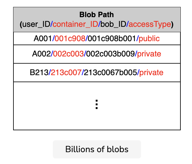
We talked about the different levels of abstraction in a blob store—the account layer, the container layer, and the blob layer. There are billions of blobs that are stored and read. There is a large number of data nodes on which we store these blobs. If we look for the data nodes that contain specific blobs out of all of the data nodes, it would be a very slow process. Instead, we can group data nodes and call each group a partition. We maintain a partition map table that contains a list of all the blobs in each partition. If we distribute the blobs on different partitions independent of their container IDs and account IDs, we encounter a problem, as shown in the following illustration:
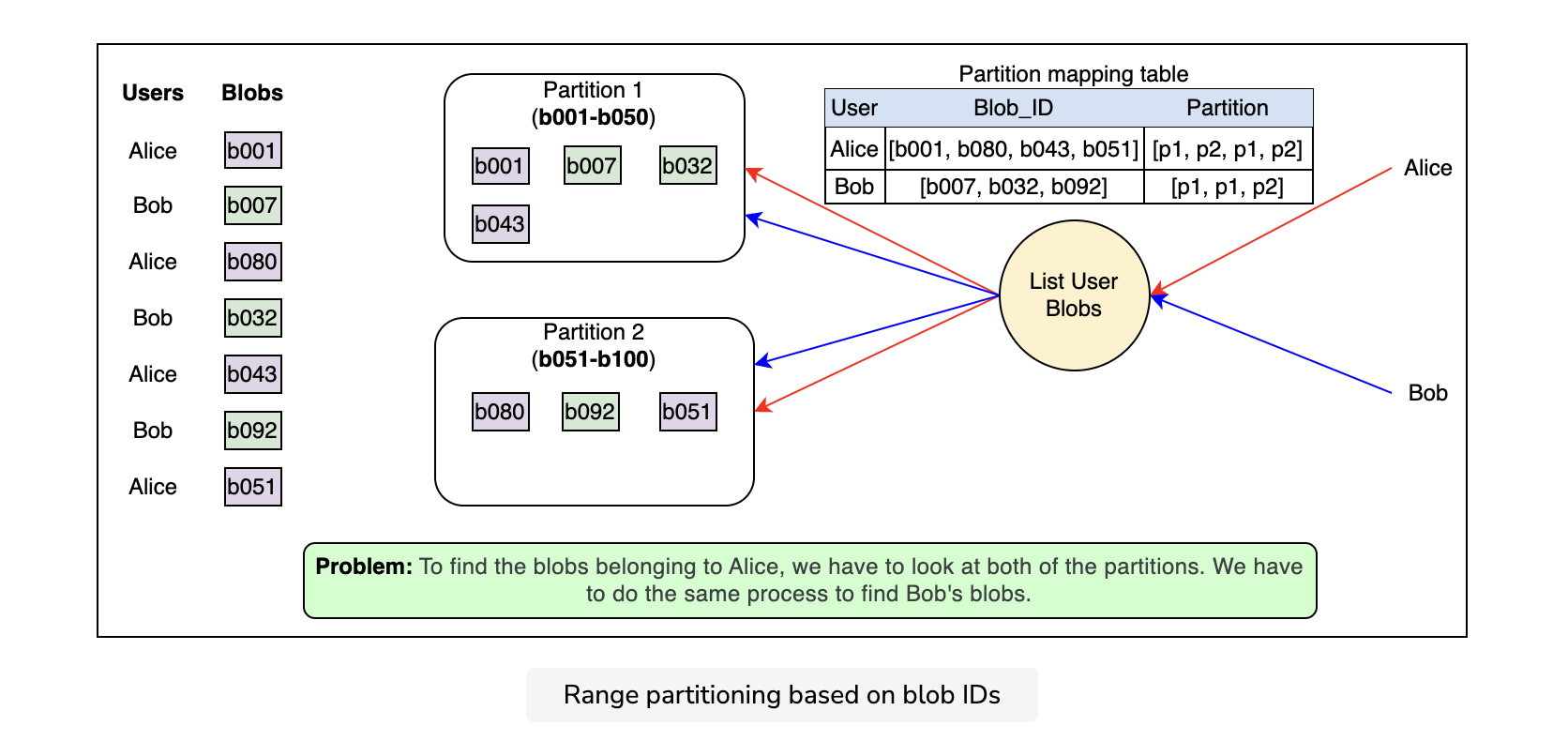
Partitioning based on the blob IDs causes certain problems. For example, the blobs under a specific container or account may reside in different partitions that add overhead while reading or listing the blobs linked to a particular account or a particular container.
To overcome the problem described above, we can partition the blobs based on the complete path of the blob. The partition key here is the combination of the account ID, container ID, and blob ID. This helps in co-locating the blobs for a single user on the same partition server, which enhances performance.
Note: The partition mappings are maintained by the manager node, and these mappings are stored in the distributed metadata storage.
Blob indexing
Finding specific blobs in a sea of blobs becomes more difficult and time-consuming with an increase in the number of blobs that are uploaded to the storage. The blob index solves the problem of blob management and querying.
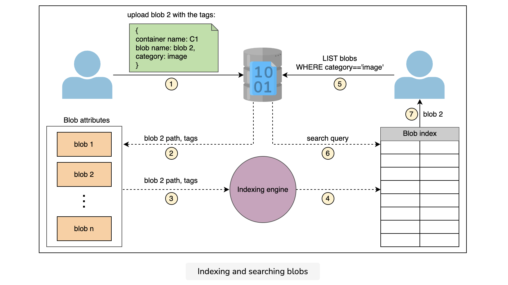
To populate the blob index, we define key-value tag attributes on the blobs while uploading the blobs. We use multiple tags, like container name, blob name, upload date and time, and some other categories like the image or video blob, and so on.
As shown in the following illustration, a blob indexing engine reads the new tags, indexes them, and exposes them to a searchable blob index:
We can categorize blobs as well as sort blobs using indexing. Let’s see how we utilize indexing in pagination.
Pagination for listing
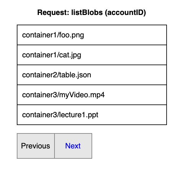
Listing is about returning a list of blobs to the user, depending on the user’s entered prefix. A prefix is a character or string that returns the blobs whose name begins with that particular character or string.
Users may want to list all the blobs associated with a specific account, all the blobs present inside a specific container, or they may want to list some public blobs based on a prefix. The problem is that this list could be very long. We can’t return the whole list to the user in one go. So, we have to return the list of the blobs in parts.
Let’s say a user wants a list of blobs associated with their account and there are a total of 2,000 blobs associated with that account. Searching, returning, and loading too many blobs at once affects performance. This is where paging becomes important. We can return the first five results and give users a next button. On each click of the next button, it returns the next five results. This is called pagination.
The application owners set the number of results to return depending on these factors:
- How much time they assume the users should wait for query response.
- How many results they can return in that time. We have shown five results per page, which is a very small number. We use this number just for visualization purposes.
Point to Ponder
Question
How do we decide which five blobs to return first out of the 2,000 blobs totalt?
Here, we utilize indexing to sort and categorize the blobs. We should do this beforehand, while we store the blobs. Otherwise, it becomes challenging at the time of returning the list to the user. There could be millions or billions of blobs and we can’t sort them quickly when the list request is received.
----------
For pagination, we need a continuation token as a starting point for the part of the list that’s returned next. A continuation token is a string token that’s included in the response of a query if the total number of queried results exceeds the maximum number of results that we can return at once. As a result, it serves as a pointer, allowing the re-query to pick up where we left off.
Replication
Replication is carried out on two levels to support availability and strong consistency. To keep the data strongly consistent, we synchronously replicate data among the nodes that are used to serve the read requests, right after performing the write operation. To achieve availability, we can replicate data to different regions or data centers after performing the write operation. We don’t serve the read request from the other data center or regions until we have not replicated data there.
These are the two levels of replication:
- Synchronous replication within a storage cluster.
- Asynchronous replication across data centers and regions.
Synchronous replication within a storage cluster
A storage cluster is made up of N racks of storage nodes, each of which is configured as a fault domain with redundant networking and power.
We ensure that every data written into a storage cluster is kept durable within that storage cluster. The manager node maintains enough data replicas across the nodes in distinct fault domains to ensure data durability inside the cluster in the event of a disk, node, or rack failure.
Note: This intra-cluster replication is done on the critical path of the client’s write requests.
Success can be returned to the client once a write has been synchronously replicated inside that storage cluster. This allows for quick writes because:
- We replicate data within a storage cluster where all the nodes are nearby, thus reducing the latency.
- We use in-lined data copying where we use redundant network paths to copy data to all the replicas in parallel.
This replication technique helps maintain data consistency and availability inside the storage cluster.
Asynchronous replication across data centers and region
The blob store’s data centers are present in different regions—for example, Asia-Pacific, Europe, eastern US, and more. In each region, we have more than one data center placed at different locations, so that if one data center goes down, we have other data centers in the same region to step in and serve the user requests. There are a minimum of three data centers within each region, each separated by miles to protect against local events like fires, floods, and so on.
The number of copies of a blob is called the replication factor. Most of the time, a replication factor of three is sufficient.
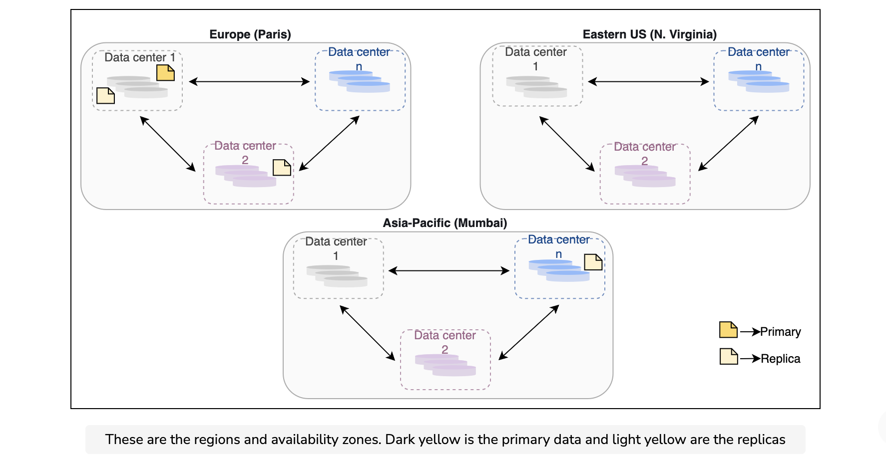
We keep four copies of a blob. One is the local copy within the data center in the primary region to protect against server rack and drive failures. The second copy of the blob is placed in the other data center within the same region to protect against fire or flooding in the data center. The third copy is placed in the data center of a different region to protect against regional disasters.
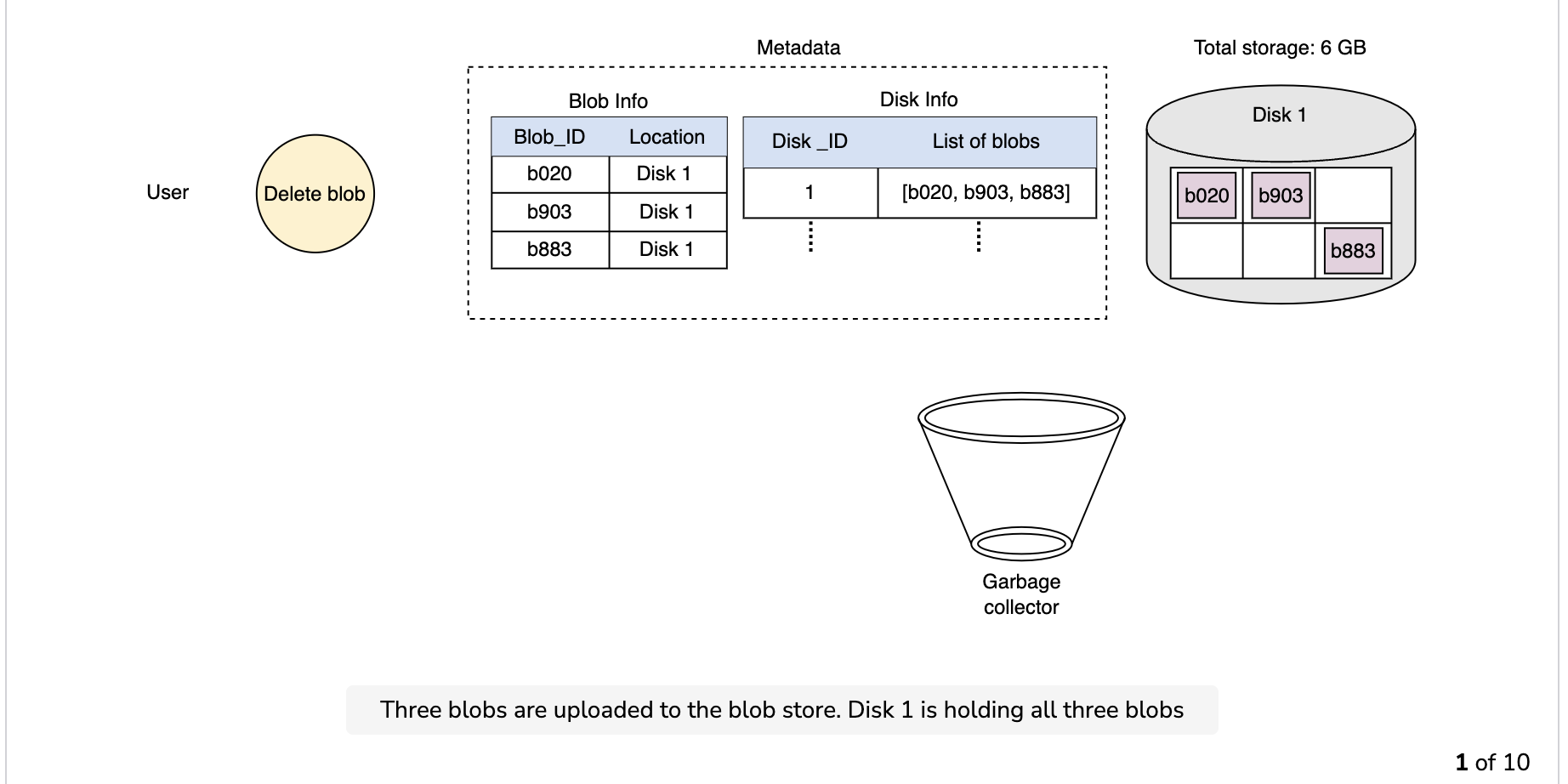
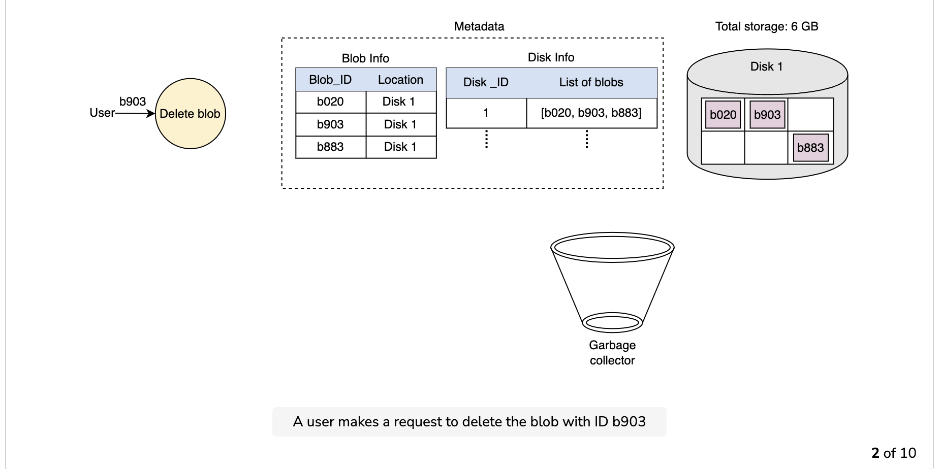
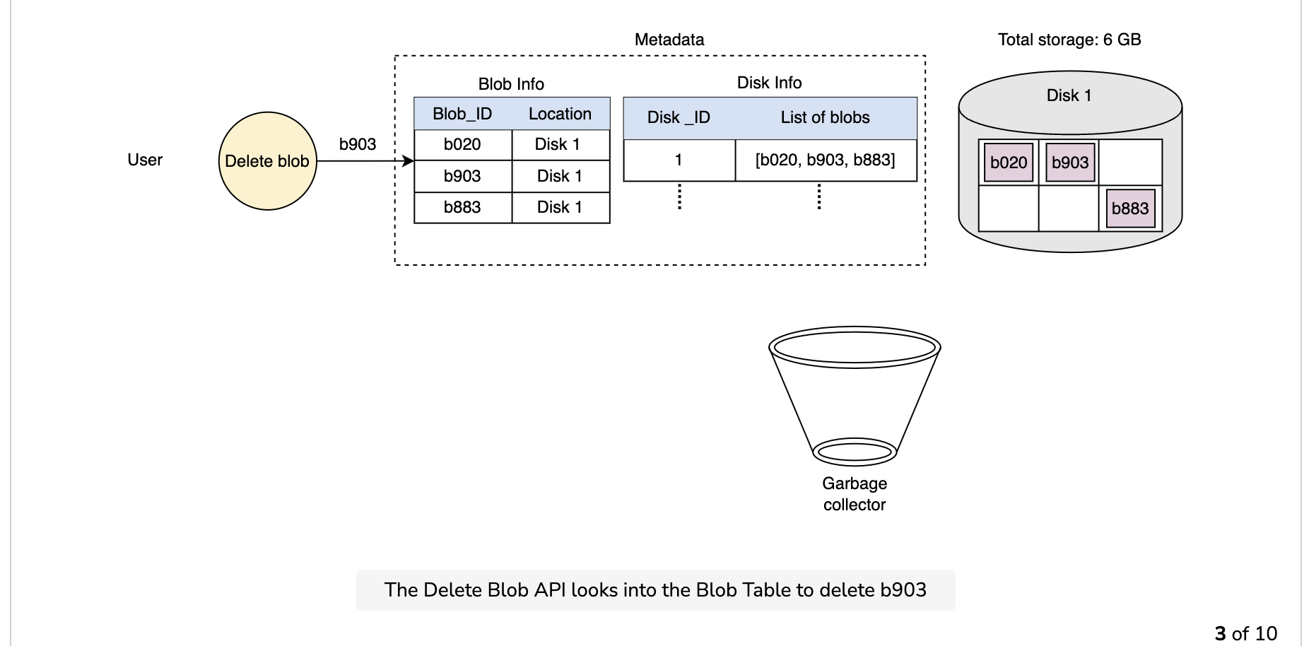
Garbage collection while deleting a blob
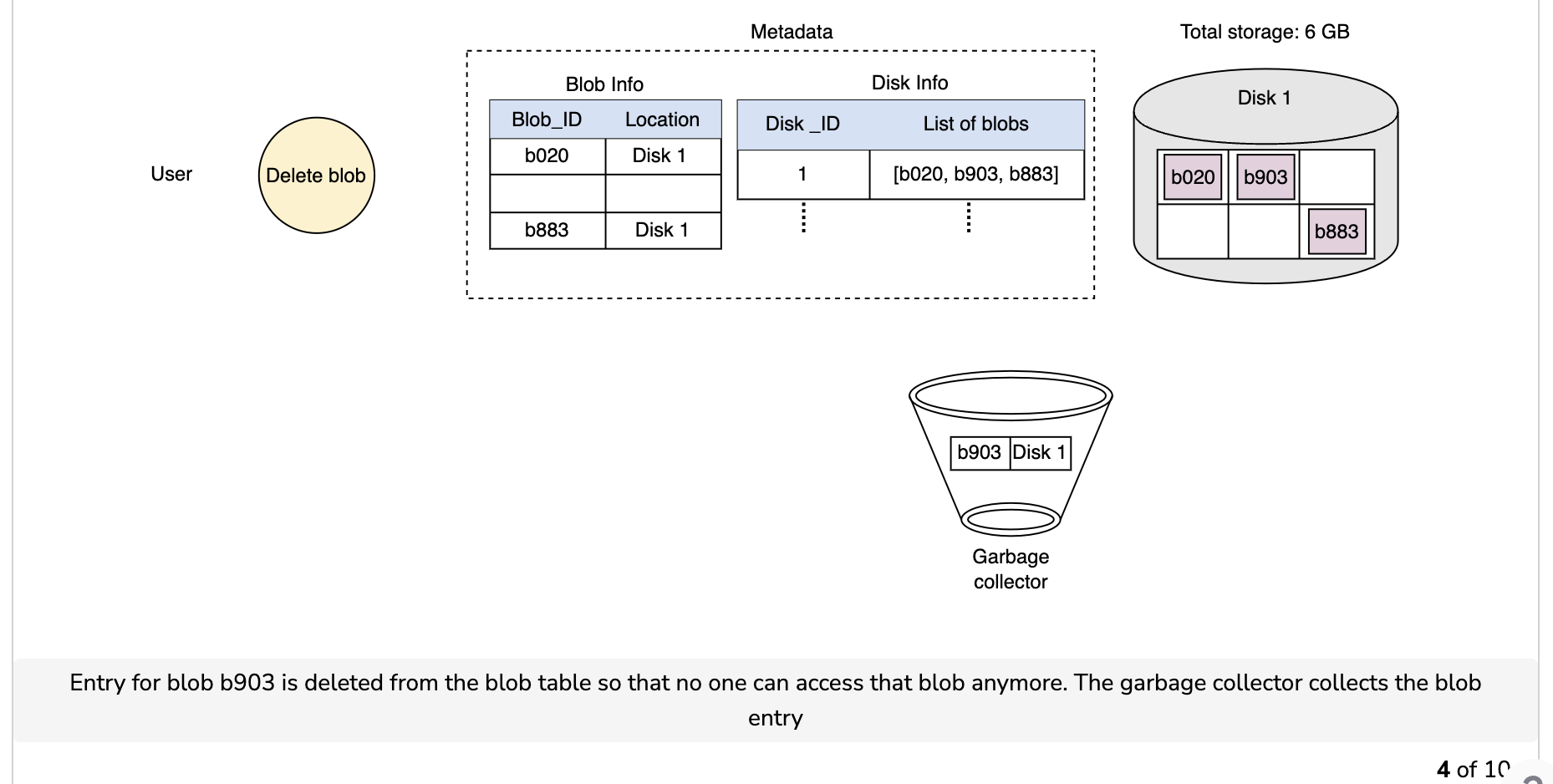
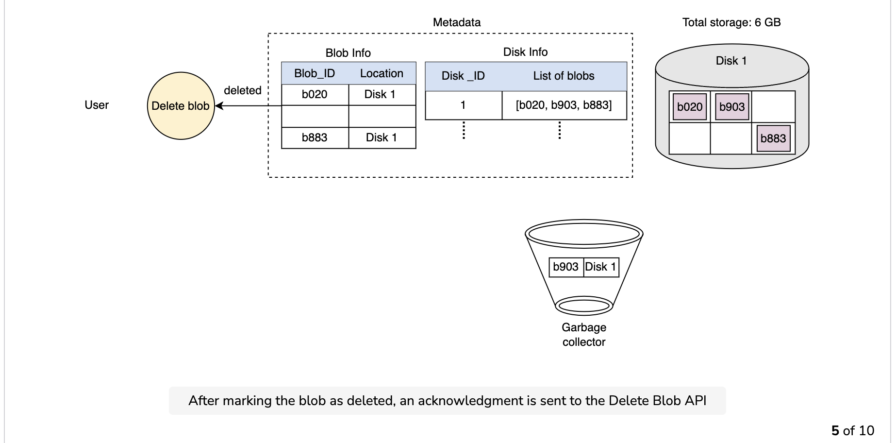
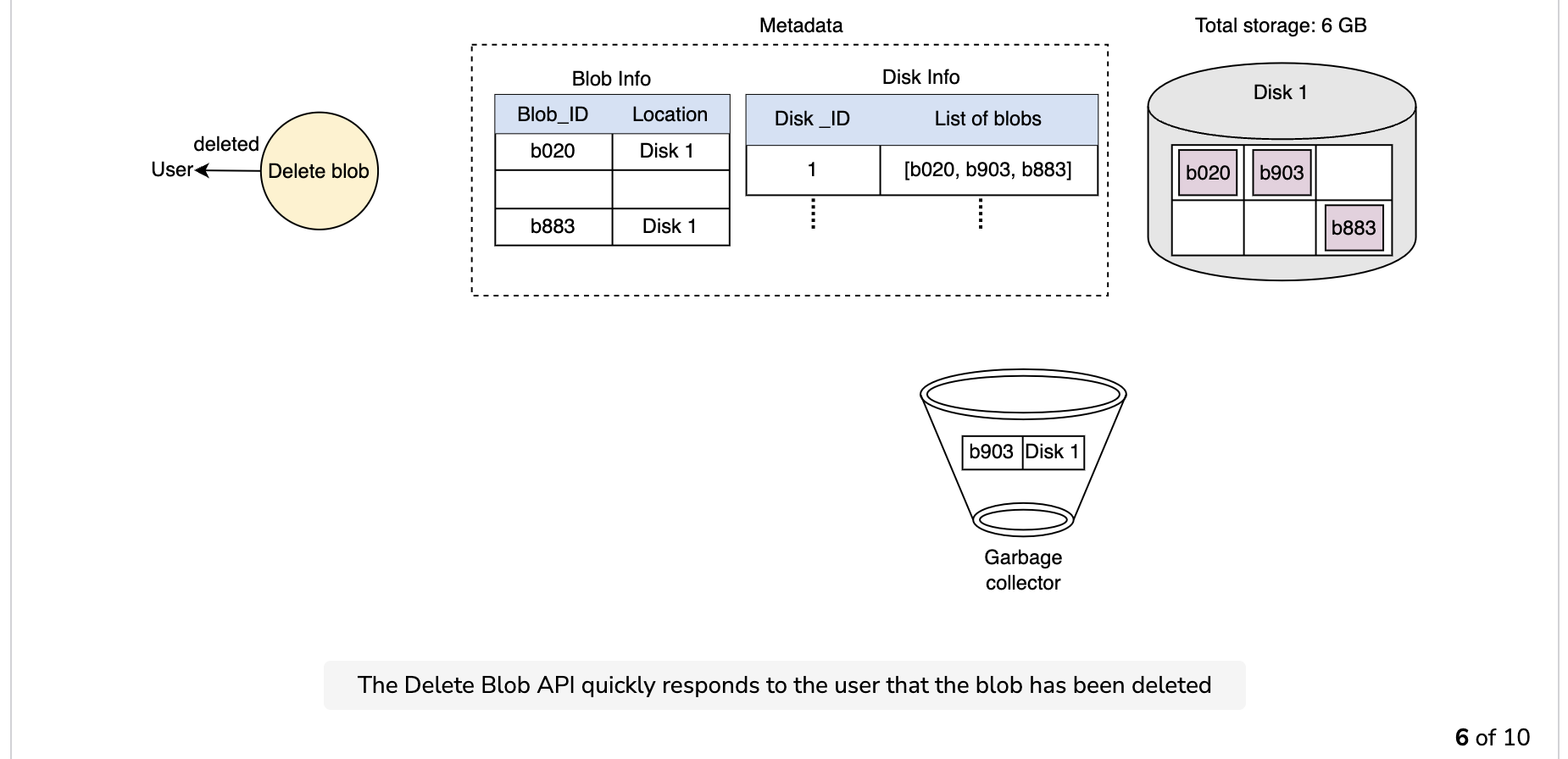
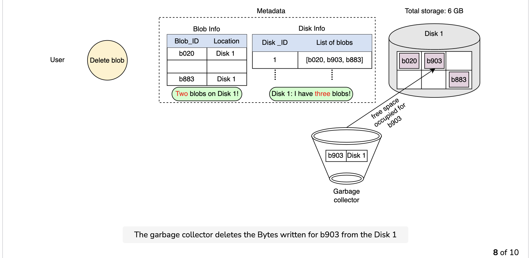
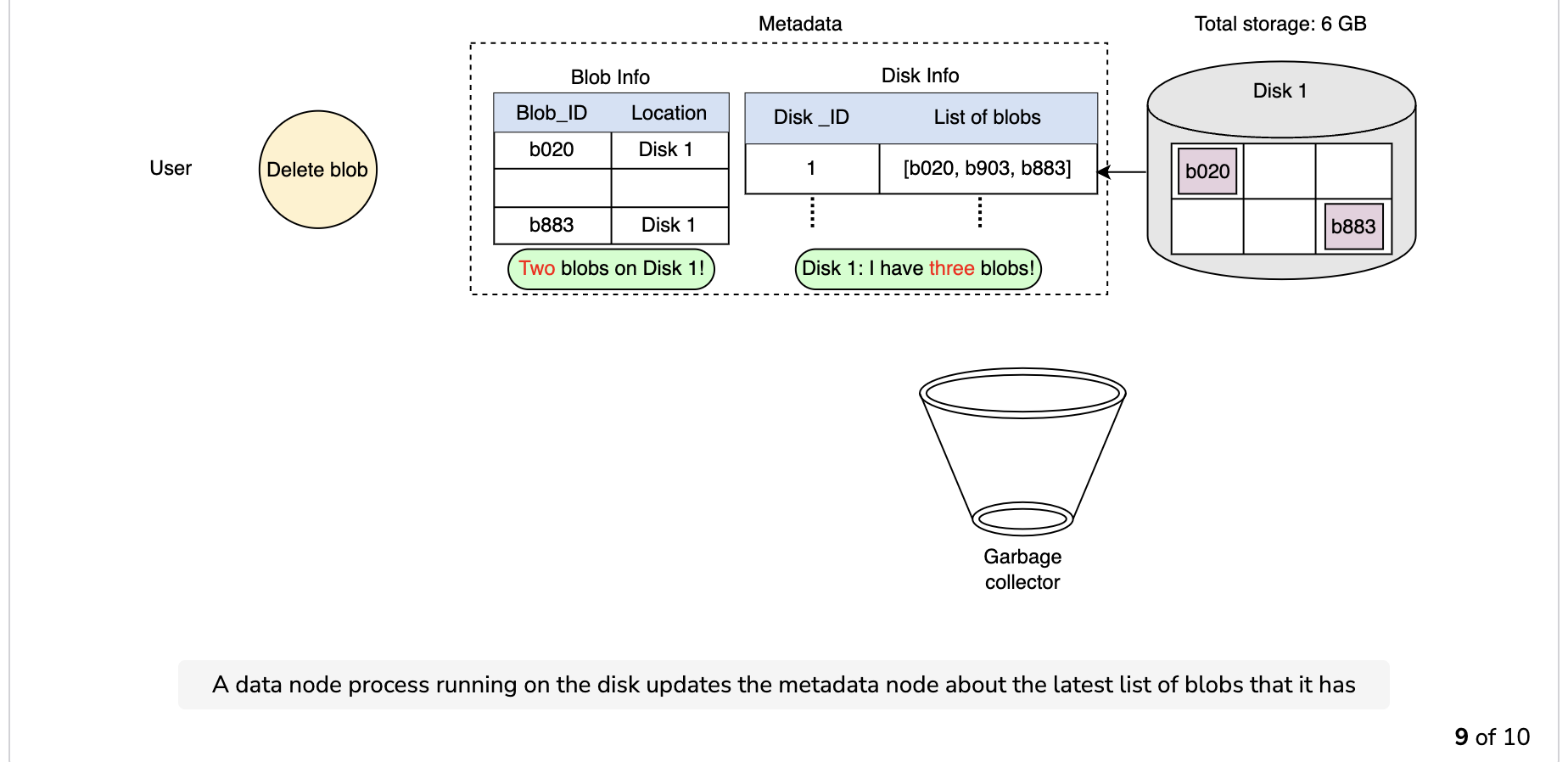
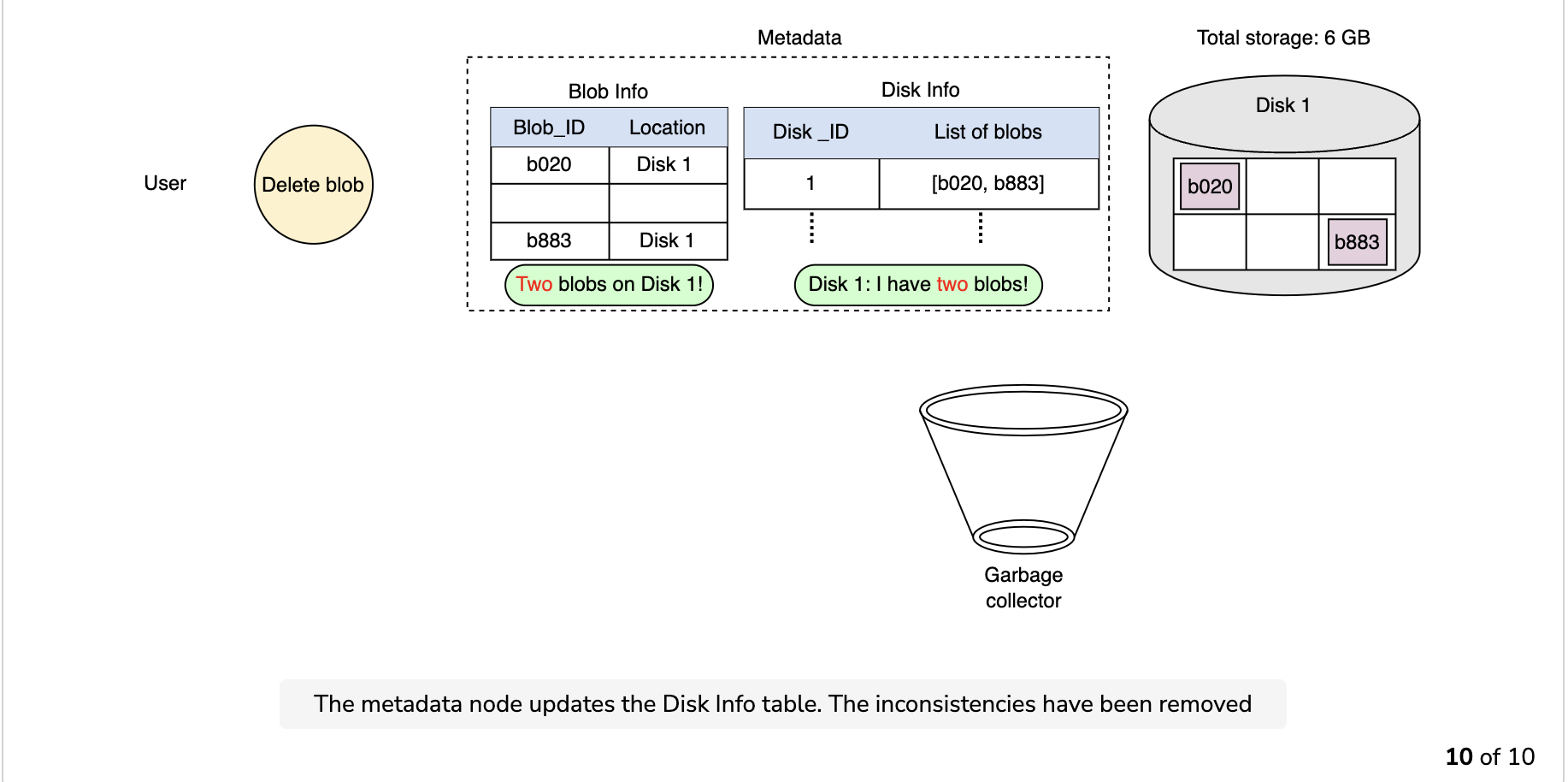
Since the blob chunks are placed at different data nodes, deleting from many different nodes takes time, and holding a client until that’s done is not a viable option. Due to real-time latency optimization, we don’t actually remove the blob from the blob store against a delete request. Instead, we just mark a blob as “DELETED” in the metadata to make it inaccessible to the user. The blob is removed later after responding to the user’s delete request.
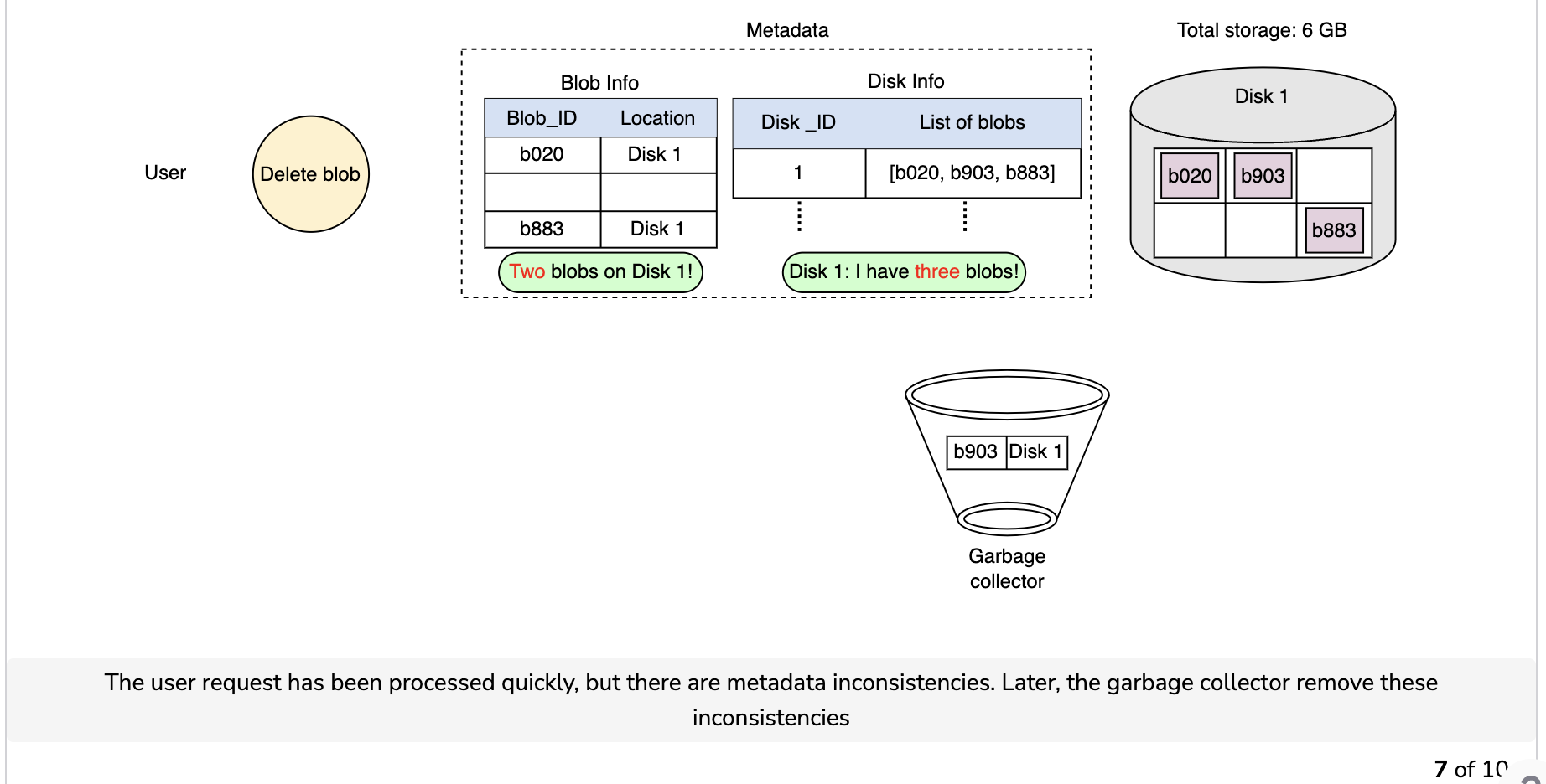
Marking the blob as deleted, but not actually deleting it at the moment, causes internal metadata inconsistencies, meaning that things continue to take up storage space that should be free. These metadata inconsistencies have no impact on the user. For example, for a blob marked as deleted in the metadata, we still have the entries for that blob’s chunks in the metadata. The data nodes are still holding on to that blob’s chunks. Therefore, we have a service called a garbage collector that cleans up metadata inconsistencies later. The deletion of a blob causes the chunks associated with that blob to be freed. However, there could be an appreciable time delay between the time a blob is deleted by a user and the time of the corresponding increase in free space in the blob store. We can bear this appreciable time delay because, in return, we have a real-time fast response benefit for the user’s delete blob request.
The whole deletion process is shown in the following illustration:
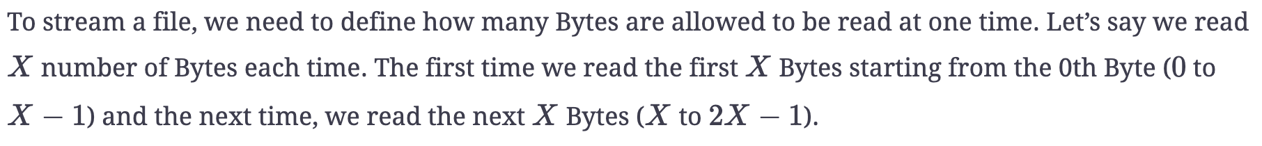
Stream a file
Question
How do we know which Bytes we have read first and which Bytes we have to read next?
We can use an offset value to keep track of the Byte from which we need to start reading again.
-------------
Cache the blob store
Caching can take place at multiple levels. Below are some examples:
- The metadata for a blob’s chunks is cached on the client side when it’s read for the first time. The client can go directly to the data nodes without communicating to the manager node to read the same blob a second time.
- At the front-end servers, we cache the partition map and use it to determine which partition server to forward each request to.
- The frequently accessed chunks are cached at the manager node, which helps us stream large objects efficiently. It also reduces disk I/O.
Note: The caching of the blob store is usually done using CDN. The Azure blob store service cache the publicly accessible blob in Azure Content Delivery Network until that blob’s TTL (time-to-live) elapses. The origin server defines the TTL, and CDN determines it from the
Cache-Controlheader in the HTTP response from the origin server.
We covered the design factors that should be taken into account while designing a blob store. Now, we’ll evaluate what we designed.